Overview
Fourier-Schur analysis is an analogue of Fourier analysis in which the time domain and corresponding cyclic symmetry are replaced by the spatial joint moment tensor domain and permutation symmetry (or, equivalently, linear spatial symmetry). It is used to derive natural higher-order statistics for “registered” spatial datasets.
The transform works by decomposing the generalized covariance tensor of several random variables into canonical components. The “sectors” (irreducible subrepresentations) defining these components in tensor space are defined a priori by the condition that they are mutually unreachable from each other by arbitrary change-of-coordinate transformations, as part of a rich theory going back to the work of Issai Schur and Hermann Weyl.
The algorithm used here is described in A Schur Transform for Spatial Stochastic Processes. See also Persi Diaconis’ Group Representations in Probability and Statistics for background on the non-abelian Fourier transform in the context of the symmetric group.
Getting started
Install from PyPI:
pip install schurtransform
Suppose that your data are stored in a multi-dimensional array data[i,j,a] (or similar list-of-list-of-lists), where
step index
iranges acrossnsteps (e.g. time-steps, or random variables)sample index
jranges crossNsamples (e.g. number of trajectories or landmarks)spatial index
aranges acrosskdimensions (e.g.k=3)
The following shows basic usage:
import schurtransform as st

data = [
    [[4,2], [4.01,2.1], [3.9,2.2]],
    [[3.99,2.1], [3.7,2.1] ,[4.0,2.2]],
    [[4.4,1.9], [4.3,1.8], [4.3,1.8]],
    [[4.6,2.0], [4.1,1.8], [4.3,1.7]],
]
decomposition = st.transform(
    samples=data,
)
print(list(decomposition.keys()))
print(decomposition['3+1'].data)
This outputs:
['1+1+1+1', '2+1+1', '2+2', '3+1', '4']

[[[[ 0.00000000e+00  4.44722222e-05]
   [ 3.48055556e-05 -3.82222222e-05]]

  [[ 2.09166667e-05  6.05555556e-05]
   [ 1.22222222e-05 -4.38888889e-05]]]


 [[[-1.00194444e-04 -1.22222222e-05]
   [-6.05555556e-05 -6.83333333e-05]]

  [[ 3.82222222e-05  5.61111111e-05]
   [ 5.61111111e-05  0.00000000e+00]]]]
The components are the GL(k)- or Sn-isotypic components of the covariance tensor of data in the tensor space with n tensor factors and k dimensions for each factor. Each one is presented as a multi-dimensional numpy array with n indices ranging across k values.
The library ships with the character tables up to S6. For more than 6-fold statistics, see Regenerating character tables for information about using GAP to generate additional character tables.
Plotting example
A more extensive usage example:
import matplotlib.pyplot as plt
import schurtransform as st
input_data = st.get_example_data(dataset = 'lung 4DCT')
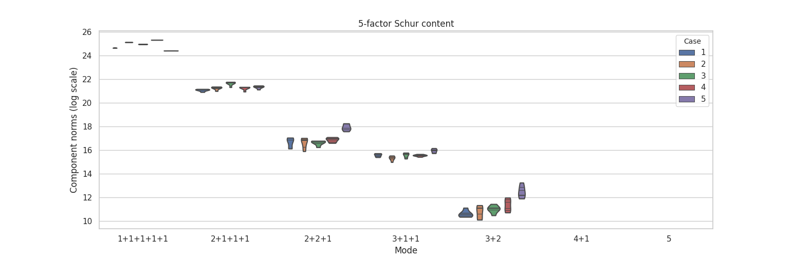
transform_data = st.transform(input_data, summary='CONTENT', number_of_factors=5)
fig1, ax1 = st.create_figure(transform_data, summary='CONTENT')
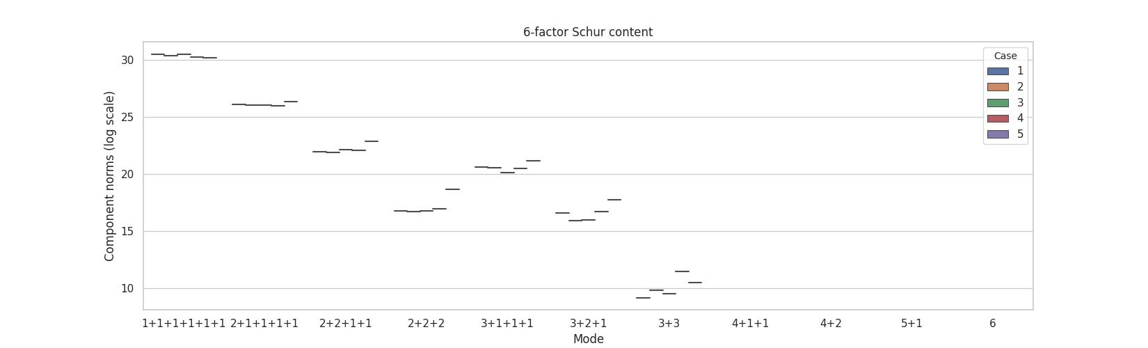
transform_data = st.transform(input_data, summary='CONTENT', number_of_factors=6)
fig2, ax2 = st.create_figure(transform_data, summary='CONTENT')
plt.show()
This calculates the Schur content (many Schur transforms for various subsets of the series index) of a lung deformation as measured by a 4D CT scan. Data available for download from DIR-lab.